3.2 Notebook
An R Notebook is an R Markdown document with chunks that can be executed independently and interactively, with output visible immediately beneath the input. See Figure 3.3 for an example.
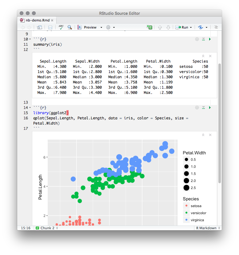
FIGURE 3.3: An R Notebook example.
R Notebooks are an implementation of Literate Programming that allows for direct interaction with R while producing a reproducible document with publication-quality output.
Any R Markdown document can be used as a notebook, and all R Notebooks can be rendered to other R Markdown document types. A notebook can therefore be thought of as a special execution mode for R Markdown documents. The immediacy of notebook mode makes it a good choice while authoring the R Markdown document and iterating on code. When you are ready to publish the document, you can share the notebook directly, or render it to a publication format with the Knit button.
3.2.1 Using Notebooks
3.2.1.1 Creating a Notebook
You can create a new notebook in RStudio with the menu command File -> New File -> R Notebook, or by using the html_notebook output type in your document’s YAML metadata.
---
title: "My Notebook"
output: html_notebook
---
By default, RStudio enables inline output (Notebook mode) on all R Markdown documents, so you can interact with any R Markdown document as though it were a notebook. If you have a document with which you prefer to use the traditional console method of interaction, you can disable notebook mode by clicking the gear button in the editor toolbar, and choosing Chunk Output in Console (Figure 3.4).
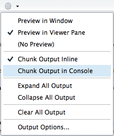
FIGURE 3.4: Send the R code chunk output to the console.
If you prefer to use the console by default for all your R Markdown documents (restoring the behavior in previous versions of RStudio), you can make Chunk Output in Console the default: Tools -> Options -> R Markdown -> Show output inline for all R Markdown documents.
3.2.1.2 Inserting chunks
Notebook chunks can be inserted quickly using the keyboard shortcut Ctrl + Alt + I (macOS: Cmd + Option + I), or via the Insert menu in the editor toolbar.
Because all of a chunk’s output appears beneath the chunk (not alongside the statement which emitted the output, as it does in the rendered R Markdown output), it is often helpful to split chunks that produce multiple outputs into two or more chunks which each produce only one output. To do this, select the code to split into a new chunk (Figure 3.5), and use the same keyboard shortcut for inserting a new code chunk (Figure 3.6).
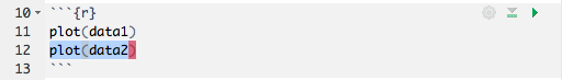
FIGURE 3.5: Select the code to split into a new chunk.
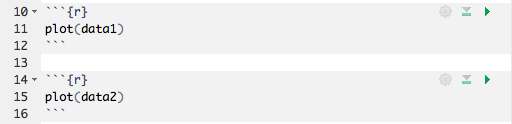
FIGURE 3.6: Insert a new chunk from the code selected before.
3.2.1.3 Executing code
Code in the notebook is executed with the same gestures you would use to execute code in an R Markdown document:
Use the green triangle button on the toolbar of a code chunk that has the tooltip “Run Current Chunk,” or
Ctrl + Shift + Enter(macOS:Cmd + Shift + Enter) to run the current chunk.Press
Ctrl + Enter(macOS:Cmd + Enter) to run just the current statement. Running a single statement is much like running an entire chunk consisting only of that statement.There are other ways to run a batch of chunks if you click the menu
Runon the editor toolbar, such asRun All,Run All Chunks Above, andRun All Chunks Below.
The primary difference is that when executing chunks in an R Markdown document, all the code is sent to the console at once, but in a notebook, only one line at a time is sent. This allows execution to stop if a line raises an error.
When you execute code in a notebook, an indicator will appear in the gutter to show you execution progress (Figure 3.7). Lines of code that have been sent to R are marked with dark green; lines that have not yet been sent to R are marked with light green. If at least one chunk is waiting to be executed, you will see a progress meter appear in the editor’s status bar, indicating the number of chunks remaining to be executed. You can click on this meter at any time to jump to the currently executing chunk. When a chunk is waiting to execute, the Run button in its toolbar will change to a “queued” icon. If you do not want the chunk to run, you can click on the icon to remove it from the execution queue.
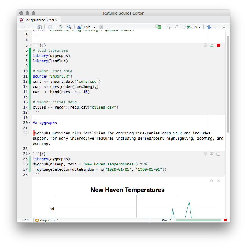
FIGURE 3.7: The indicator in the gutter to show the execution progress of a code chunk in the notebook.
In general, when you execute code in a notebook chunk, it will do exactly the same thing as it would if that same code were typed into the console. There are however a few differences:
Output: The most obvious difference is that most forms of output produced from a notebook chunk are shown in the chunk output rather than, for example, the RStudio Viewer or the Plots pane. Console output (including warnings and messages) appears both at the console and in the chunk output.
Working directory: The current working directory inside a notebook chunk is always the directory containing the notebook
.Rmdfile. This makes it easier to use relative paths inside notebook chunks, and also matches the behavior when knitting, making it easier to write code that works identically both interactively and in a standalone render.You’ll get a warning if you try to change the working directory inside a notebook chunk, and the directory will revert back to the notebook’s directory once the chunk is finished executing. You can suppress this warning by using the
warnings = FALSEchunk option.If it is necessary to execute notebook chunks in a different directory, you can change the working directory for all your chunks by using the knitr
root.diroption. For instance, to execute all notebook chunks in the grandparent folder of the notebook:knitr::opts_knit$set(root.dir = normalizePath(".."))This option is only effective when used inside the setup chunk. Also note that, as in knitr, the
root.dirchunk option applies only to chunks; relative paths in Markdown are still relative to the notebook’s parent folder.Warnings: Inside a notebook chunk, warnings are always displayed immediately rather than being held until the end, as in
options(warn = 1).Plots: Plots emitted from a chunk are rendered to match the width of the editor at the time the chunk was executed. The height of the plot is determined by the golden ratio. The plot’s display list is saved, too, and the plot is re-rendered to match the editor’s width when the editor is resized.
You can use the
fig.width,fig.height, andfig.aspchunk options to manually specify the size of rendered plots in the notebook; you can also useknitr::opts_chunk$set(fig.width = ..., fig.height = ...)in the setup chunk to to set a default rendered size. Note, however, specifying a chunk size manually suppresses the generation of the display list, so plots with manually specified sizes will be resized using simple image scaling when the notebook editor is resized.
To execute an inline R expression in the notebook, put your cursor inside the chunk and press Ctrl + Enter (macOS: Cmd + Enter). As in the execution of ordinary chunks, the content of the expression will be sent to the R console for evaluation. The results will appear in a small pop-up window next to the code (Figure 3.8).
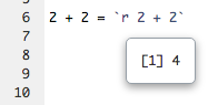
FIGURE 3.8: Output from an inline R expression in the notebook.
In notebooks, inline R expressions can only produce text (not figures or other kinds of output). It is also important that inline R expressions executes quickly and do not have side-effects, as they are executed whenever you save the notebook.
Notebooks are typically self-contained. However, in some situations, it is preferable to re-use code from an R script as a notebook chunk, as in knitr’s code externalization. This can be done by using knitr::read_chunk() in your notebook’s setup chunk, along with a special ## ---- chunkname annotation in the R file from which you intend to read code. Here is a minimal example with two files:
example.Rmd
```{r setup}
knitr::read_chunk("example.R")
```
example.R
## ---- chunk
1 + 1
When you execute the empty chunk in the notebook example.Rmd, code from the external file example.R will be inserted, and the results displayed inline, as though the chunk contained that code (Figure 3.9).
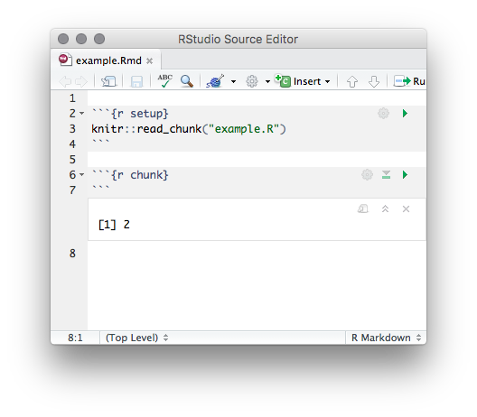
FIGURE 3.9: Execute a code chunk read from an external R script.
3.2.1.4 Chunk output
When code is executed in the notebook, its output appears beneath the code chunk that produced it. You can clear an individual chunk’s output by clicking the X button in the upper right corner of the output, or collapse it by clicking the chevron.
It is also possible to clear or collapse all of the output in the document at once using the Collapse All Output and Clear All Output menu items available on the gear menu in the editor toolbar (Figure 3.4).
If you want to fully reset the state of the notebook, the item Restart R and Clear Output on the Run menu on the editor toolbar will do the job.
Ordinary R Markdown documents are “knitted,” but notebooks are “previewed.” While the notebook preview looks similar to a rendered R Markdown document, the notebook preview does not execute any of your R code chunks. It simply shows you a rendered copy of the Markdown output of your document along with the most recent chunk output. This preview is generated automatically whenever you save the notebook (whether you are viewing it in RStudio or not); see the section beneath on the *.nb.html file for details.
When html_notebook is the topmost (default) format in your YAML metadata, you will see a Preview button in the editor toolbar. Clicking it will show you the notebook preview (Figure 3.10).
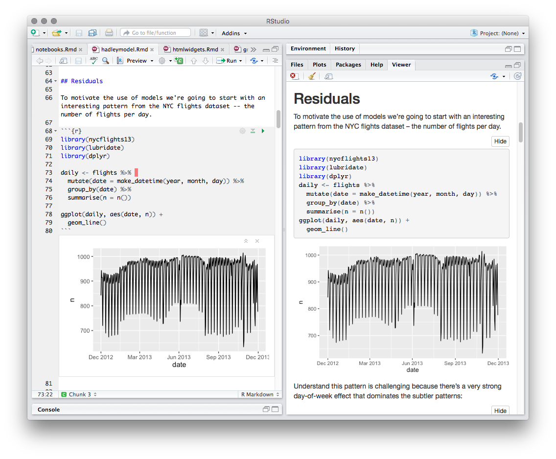
FIGURE 3.10: Preview a notebook.
If you have configured R Markdown previewing to use the Viewer pane (as illustrated in Figure 3.10), the preview will be automatically updated whenever you save your notebook.
When an error occurs while a notebook chunk is executing (Figure 3.11):
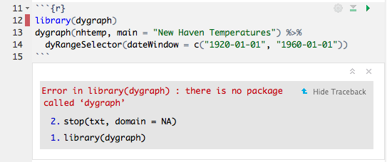
FIGURE 3.11: Errors in a notebook.
Execution will stop; the remaining lines of that chunk (and any chunks that have not yet been run) will not be executed.
The editor will scroll to the error.
The line of code that caused the error will have a red indicator in the editor’s gutter.
If you want your notebook to keep running after an error, you can suppress the first two behaviors by specifying error = TRUE in the chunk options.
In most cases, it should not be necessary to have the console open while using the notebook, as you can see all of the console output in the notebook itself. To preserve vertical space, the console will be automatically collapsed when you open a notebook or run a chunk in the notebook.
If you prefer not to have the console hidden when chunks are executed, uncheck the option from the menu Tools -> Global Options -> R Markdown -> Hide console automatically when executing notebook chunks.
3.2.2 Saving and sharing
3.2.2.1 Notebook file
When a notebook *.Rmd file is saved, a *.nb.html file is created alongside it. This file is a self-contained HTML file which contains both a rendered copy of the notebook with all current chunk outputs (suitable for display on a website) and a copy of the *.Rmd file itself.
You can view the *.nb.html file in any ordinary web browser. It can also be opened in RStudio; when you open there (e.g., using File -> Open File), RStudio will do the following:
Extract the bundled
*.Rmdfile, and place it alongside the*.nb.htmlfile.Open the
*.Rmdfile in a new RStudio editor tab.Extract the chunk outputs from the
*.nb.htmlfile, and place them appropriately in the editor.
Note that the *.nb.html file is only created for R Markdown documents that are notebooks (i.e., at least one of their output formats is html_notebook). It is possible to have an R Markdown document that includes inline chunk output beneath code chunks, but does not produce an *.nb.html file, when html_notebook is not specified as an output format for the R Markdown document.
3.2.2.2 Output storage
The document’s chunk outputs are also stored in an internal RStudio folder beneath the project’s .Rproj.user folder. If you work with a notebook but do not have a project open, the outputs are stored in the RStudio state folder in your home directory (the location of this folder varies between the desktop and the server).
3.2.2.3 Version control
One of the major advantages of R Notebooks compared to other notebook systems is that they are plain-text files and therefore work well with version control. We recommend checking in both the *.Rmd and *.nb.html files into version control, so that both your source code and output are available to collaborators. However, you can choose to include only the *.Rmd file (with a .gitignore that excludes *.nb.html) if you want each collaborator to work with their own private copies of the output.
3.2.3 Notebook format
While RStudio provides a set of integrated tools for authoring R Notebooks, the notebook file format itself is decoupled from RStudio. The rmarkdown package provides several functions that can be used to read and write R Notebooks outside of RStudio.
In this section, we describe the internals of the notebook format. It is primarily intended for front-end applications using or embedding R, or other users who are interested in reading and writing documents using the R Notebook format. We recommend that beginners skip this section when reading this book or using notebooks for the first time.
R Notebooks are HTML documents with data written and encoded in such a way that:
The source Rmd document can be recovered, and
Chunk outputs can be recovered.
To generate an R Notebook, you can use rmarkdown::render() and specify the html_notebook output format in your document’s YAML metadata. Documents rendered in this form will be generated with the .nb.html file extension, to indicate that they are HTML notebooks.
To ensure chunk outputs can be recovered, the elements of the R Markdown document are enclosed with HTML comments, providing more information on the output. For example, chunk output might be serialized in the form:
<!-- rnb-chunk-begin -->
<!-- rnb-output-begin -->
<pre><code>Hello, World!</code></pre>
<!-- rnb-output-end -->
<!-- rnb-chunk-end -->
Because R Notebooks are just HTML documents, they can be opened and viewed in any web browser; in addition, hosting environments can be configured to recover and open the source Rmd document, and also recover and display chunk outputs as appropriate.
3.2.3.1 Generating R Notebooks with custom output
It is possible to render an HTML notebook with custom chunk outputs inserted in lieu of the result that would be generated by evaluating the associated R code. This can be useful for front-end editors that show the output of chunk execution inline, or for conversion programs from other notebook formats where output is already available from the source format. To facilitate this, one can provide a custom “output source” to rmarkdown::render(). Let’s investigate with a simple example:
rmd_stub = "examples/r-notebook-stub.Rmd"
cat(readLines(rmd_stub), sep = "\n")
---
title: "R Notebook Stub"
output: html_notebook
---
```{r chunk-one}
print("Hello, World!")
```Let’s try to render this document with a custom output source, so that we can inject custom output for the single chunk within the document. The output source function will accept:
code: The code within the current chunk.context: An environment containing active chunk options and other chunk information....: Optional arguments reserved for future expansion.
In particular, the context elements label and chunk.index can be used to help identify which chunk is currently being rendered.
output_source = function(code, context, ...) {
  logo = file.path(R.home("doc"), "html", "logo.jpg")
  if (context$label == "chunk-one") list(
    rmarkdown::html_notebook_output_code("# R Code"),
    paste("Custom output for chunk:", context$chunk.index),
    rmarkdown::html_notebook_output_code("# R Logo"),
    rmarkdown::html_notebook_output_img(logo)
  )
}
We can pass our output_source along as part of the output_options list to rmarkdown::render().
output_file = rmarkdown::render(
  rmd_stub,
  output_options = list(output_source = output_source),
  quiet = TRUE
)
## Warning in eng_r(options): Failed to tidy R code in chunk 'chunk-one'. Reason:
## Error : The formatR package is required by the chunk option tidy = TRUE but not installed; tidy = TRUE will be ignored.We have now generated an R Notebook. Open this document in a web browser, and it will show that the output_source function has effectively side-stepped evaluation of code within that chunk, and instead returned the injected result.
3.2.3.2 Implementing output sources
In general, you can provide regular R output in your output source function, but rmarkdown also provides a number of endpoints for insertion of custom HTML content. These are documented within ?html_notebook_output.
Using these functions ensures that you produce an R Notebook that can be opened in R frontends (e.g., RStudio).
3.2.3.3 Parsing R Notebooks
The rmarkdown::parse_html_notebook() function provides an interface for recovering and parsing an HTML notebook.
parsed = rmarkdown::parse_html_notebook(output_file)
str(parsed, width = 60, strict.width = 'wrap')
List of 4
$ source : chr [1:294] "<!DOCTYPE html>" "" "<html>" "" ...
$ rmd : chr [1:8] "---" "title: \"R Notebook Stub\""
"output: html_notebook" "---" ...
$ header : chr [1:180] "<head>" "" "<meta charset=\"utf-8\"
/>" "<meta name=\"generator\" content=\"pandoc\" />" ...
$ annotations:List of 12
..$ :List of 4
.. ..$ row : int 213
.. ..$ label: chr "text"
.. ..$ state: chr "begin"
.. ..$ meta : NULL
..$ :List of 4
.. ..$ row : int 214
.. ..$ label: chr "text"
.. ..$ state: chr "end"
.. ..$ meta : NULL
..$ :List of 4
.. ..$ row : int 215
.. ..$ label: chr "chunk"
.. ..$ state: chr "begin"
.. ..$ meta : NULL
..$ :List of 4
.. ..$ row : int 216
.. ..$ label: chr "source"
.. ..$ state: chr "begin"
.. ..$ meta :List of 1
.. .. ..$ data: chr "```r\n# R Code\n```"
..$ :List of 4
.. ..$ row : int 218
.. ..$ label: chr "source"
.. ..$ state: chr "end"
.. ..$ meta : NULL
..$ :List of 4
.. ..$ row : int 219
.. ..$ label: chr "output"
.. ..$ state: chr "begin"
.. ..$ meta :List of 1
.. .. ..$ data: chr "Custom output for chunk: 1\n"
..$ :List of 4
.. ..$ row : int 221
.. ..$ label: chr "output"
.. ..$ state: chr "end"
.. ..$ meta : NULL
..$ :List of 4
.. ..$ row : int 222
.. ..$ label: chr "source"
.. ..$ state: chr "begin"
.. ..$ meta :List of 1
.. .. ..$ data: chr "```r\n# R Logo\n```"
..$ :List of 4
.. ..$ row : int 224
.. ..$ label: chr "source"
.. ..$ state: chr "end"
.. ..$ meta : NULL
..$ :List of 4
.. ..$ row : int 225
.. ..$ label: chr "plot"
.. ..$ state: chr "begin"
.. ..$ meta : NULL
..$ :List of 4
.. ..$ row : int 227
.. ..$ label: chr "plot"
.. ..$ state: chr "end"
.. ..$ meta : NULL
..$ :List of 4
.. ..$ row : int 228
.. ..$ label: chr "chunk"
.. ..$ state: chr "end"
.. ..$ meta : NULLThis interface can be used to recover the original Rmd source, and also (with some more effort from the front-end) the ability to recover chunk outputs from the document itself.